First, fix the direction of the pair
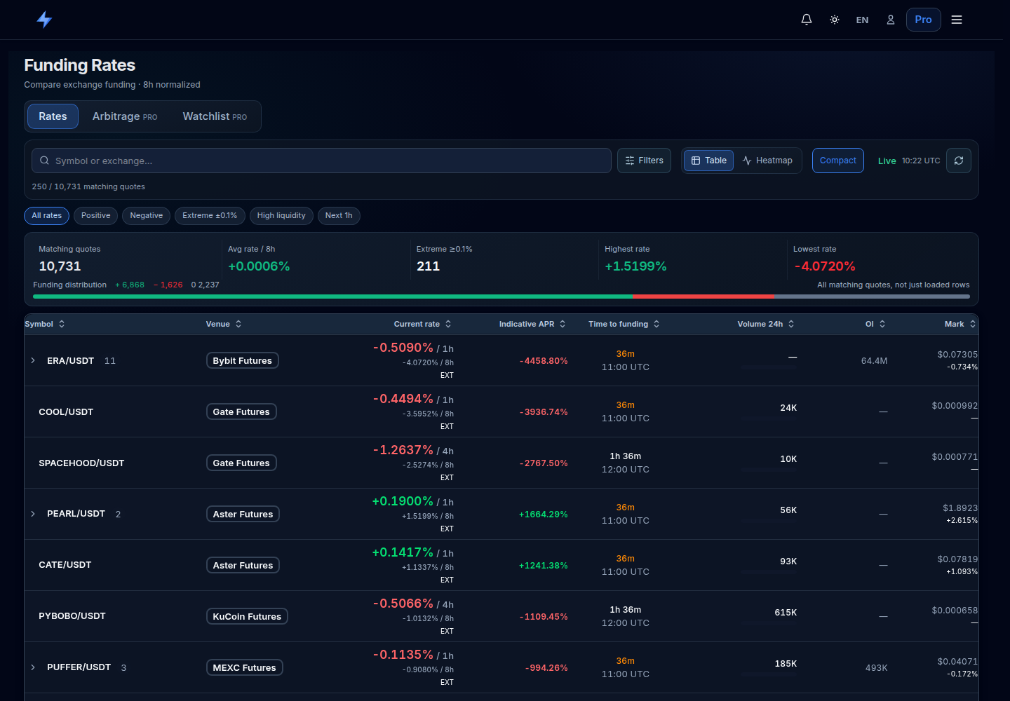
In Funding, open the Arbitrage tab, choose a pair and open its chart. In the paired rate view, expand “Rate differential.” It shows the mean, median, positive intervals, sign changes and history coverage. Pair research belongs to the Pro section; the table of individual rates, Rates, is free.
Identify the long venue and the short venue. For that direction, the differential is the short-venue rate minus the long-venue rate. Swapping the legs reverses its sign. The comparison applies to the chosen asset and comparable contracts.
History first answers: “What did this differential look like in the available observations?” To answer “What would a trade have earned?” you also need actual settlements, notionals, holding times, fills and costs.
 Open the original in a new tab
Why history uses eight-hour normalized rates
The same numerical rate over different intervals does not represent the same funding flow. Pair research compares rates normalized to eight hours. This is a comparison unit; it does not change a venue’s actual settlement schedule.
Worked interval normalization
Suppose the short venue quotes +0.006% for one hour and the long venue +0.010% for eight hours. Linear normalization gives 0.006% × 8 = 0.048% per eight hours. The differential is 0.048% − 0.010% = +0.038 percentage points per eight hours, displayed as +0.0380% in the interface.
This compares the observed rates. The same total flow over the next eight hours would require additional assumptions: unchanged rates and notionals, participation in every settlement and the relevant schedule. Observation history does not guarantee those conditions.
Check each venue’s original interval and next settlement before evaluating a trade. For example, Hyperliquid describes hourly payments with an eight-hour rate formula. Bybit explains that the quoted rate changes before settlement and settlement frequency can be adjusted.
Mean, median and sign changes in one example
Take a fully elapsed 10:00–10:30 UTC window. Below are illustrative interval-average rates, already normalized to eight hours. This is a constructed dataset for checking the arithmetic, not market history.
| UTC | Long rate | Short rate | Differential |
|---|---|---|---|
| 10:00–10:05 | +0.0100% | +0.0300% | +0.0200% |
| 10:05–10:10 | +0.0100% | +0.0200% | +0.0100% |
| 10:10–10:15 | +0.0200% | +0.0100% | −0.0100% |
| 10:15–10:20 | — | +0.0150% | — |
| 10:20–10:25 | +0.0100% | +0.0100% | 0.0000% |
| 10:25–10:30 | +0.0100% | +0.0300% | +0.0200% |
Five of the six expected intervals have both legs. The differentials entering the calculation are +0.0200%, +0.0100%, −0.0100%, 0.0000% and +0.0200%.
- Mean: +0.0080%
- The five differentials sum to +0.0400%; divide by 5. Each shared five-minute interval receives equal weight. This is the average observed differential, not a half-hour return.
- Median: +0.0100%
- Sorted values are −0.0100%, 0.0000%, +0.0100%, +0.0200%, +0.0200%. The median is the middle value. With an even number of intervals, it is the average of the two middle values.
- Positive intervals: 60%
- Three of five available values are strictly above zero: 3 / 5 × 100 = 60%. Zero counts as an observation but not a positive one. The missing interval enters neither the numerator nor the denominator of this statistic.
- Sign changes: 1
- The differential moves from positive to negative between the adjacent 10:05–10:10 and 10:10–10:15 intervals. No comparison is made across a gap. Zero also does not form a direct positive-to-negative or negative-to-positive transition: a “positive, zero, negative” sequence would count as 0 such changes here.
- Coverage: 83.3%
- There are five shared intervals out of six expected: 5 / 6 × 100 ≈ 83.3%. Unlike the positive percentage, coverage includes expected intervals without a pair of observations in its denominator.
Another worked example: differentials of 0.01%, 0.01%, 0.01%, 0.01% and 0.16% give a mean of 0.04% but a median of 0.01%. One large value materially lifts the mean. Compare both statistics and the history shape, rather than choosing only the most attractive number.
Complete history and a recent record answer different questions
Coverage tells you what share of expected completed intervals has both legs. It does not grade the accuracy of exchange data or establish that every second was observed. Even 100% coverage does not turn a past differential into a forecast.
The positive percentage describes only the available sample. In a teaching example, two positive intervals are available out of twelve expected. Positive intervals are 100%, while coverage displays only 16.6% because the interface rounds coverage down. The other ten intervals remain unknown.
“Latest record” is shown separately for the long and short legs. If one venue updated a minute ago and the other twenty minutes ago, one leg is delayed. A fresh record can belong to an unfinished interval and therefore not yet enter the shared statistics.
Use the same period when comparing pairs, and read coverage alongside the number of shared intervals. Statistics from a few scattered observations and from a continuously available history have different evidential foundations.
Why you cannot sum observations as payments
A rate can be observed every five minutes even when the contract settles once every several hours. Summing the same eight-hour rate from all five-minute observations would repeatedly count the same possible settlement. Neither the mean nor the positive percentage measures a return on capital.
Actual funding requires a separate settlement record for each leg: time, final rate, participating position value and payment currency. The funding mechanics guide explains payment directions. Different venue schedules can produce cash flows at different times.
A trade’s result is both legs’ price P&L plus actual funding, less fees and other costs. In a pre-trade estimate, include slippage relative to quotes; when using actual fill prices, that effect is already included in price P&L and must not be subtracted again. Assess the margin buffer on each venue separately. A positive differential history does not remove basis or liquidation risk; see the hedging guide and the leverage and margin explanation.
How to repeat the review for a pair
- In Arbitrage, choose the asset, long venue and short venue. Open the paired rate chart and expand “Rate differential.”
- Fix the period. First read the history status, both latest-record ages and the number of shared intervals.
- Compare mean and median. Check whether one unusual value dominates your impression of the history.
- Read the positive percentage, sign changes and chart gaps together. Do not extend the conclusion to missing intervals.
- Check the current intervals and final payments on the exchanges. Assess execution, costs and margin separately from descriptive rate statistics.
Open Funding pair research — Pro
To explore individual rates, open the free Rates table. It helps you choose markets to study; a particular pair’s available history depends on recorded observations.
For an example using saved market data, read the October 18, 2026 BTC funding-history review for Binance and Bybit. It distinguishes those observations from the teaching values in this guide.
Sources and method
The intervals and statistics were checked against VoltArb’s pair-research calculation and interface on October 18, 2026. The teaching datasets are constructed to make the calculation reproducible; they do not represent a pair’s historical returns.
Rate changes and settlement-schedule differences were checked against the official Bybit and Hyperliquid material linked above. For a particular contract, use its venue’s current rules and confirmed settlements.